
Introduction to Machine Learning (Topics 19 - 24)
19. The Basic Concept of Swarm Intelligence
Swarm intelligence is a biologically inspired approach that models the collective behavior of decentralized, self-organized systems such as insect colonies, bird flocks, or fish schools. It focuses on simple rules and interactions among individuals to solve complex problems.
This approach underlies algorithms such as Particle Swarm Optimization (PSO) and Ant Colony Optimization (ACO), which capitalize on principles of cooperation, competition, and group dynamics to explore solution spaces efficiently. Swarm intelligence provides adaptable, scalable problem-solving methods robust against dynamic system changes, reflecting its biological inspirations.
Characteristics
- Decentralization: A collective system capable of performing complex tasks in a dynamic and changing environment without any external control or central coordination
- Self-organization: Collective behavior emerges from simple interactions.
- Adaptability: Swarms can dynamically adjust to changing environments.
- Robustness: The system can function even when some individuals fail.
Mechanisms in Swarm Intelligence
- Simple Behaviors: Individual agents follow basic rules that can lead to complex group behavior.
- Massive Number of Agents: Large populations contribute to the robustness and effectiveness of the system.
- Continuous Operations: The collective is capable of ongoing function without central intervention.
- Graceful Degradation: Performance degrades gradually rather than failing abruptly when agents are removed, potentially withstands removal of large numbers of agents.
Applications
- Ant Colony Optimization (ACO): Solves optimization problems by mimicking how ants find paths to food.
- Particle Swarm Optimization (PSO): Models social behavior to find optimal solutions in complex search spaces.
Key Points
- Swarm intelligence captures the emergent behavior of natural systems through simple rules and interactions.
- It utilizes the massive parallelism and redundancy of large groups of agents.
- Provides efficient, adaptable solutions for optimization and control problems.
20. Optimization by Particle Swarm Optimization
Particle Swarm Optimization (PSO) is a nature-inspired method drawing from the social behavior of bird flocks or fish schools to optimize complex functions. Each solution, represented as a particle, navigates the search space, influenced by its previous best and group-best solutions, achieving convergence through cooperative dynamics.
PSO updates particle positions and velocities using relationships with personal and neighborhood best positions, optimizing solutions while maintaining diversity. Its capacity for exploring and exploiting search areas efficiently makes PSO applicable to diverse problems, while potential stagnation issues require strategies like inertia weight adjustments to maintain global search capabilities.
General idea
- PSO applies the concept of social interaction to problem solving
- It uses a number of so-called particles that move in swarms in the search space in search of the best solution
- It treats each particle as a spatial point, which adjusts its "flight" based on its own flight experience as well as the flight experience of other particles
Key Concepts
- Particles: Each particle represents a potential solution.
- Velocity and Position: Particles move through the solution space, adjusting their position based on their velocity.
- Personal and Global Best (pbest, gbest): Each particle retains information about its best position, and the swarm tracks the best known global position.
- pbest: The best position the particle has found so far.
- gbest: The best position found by any particle in the swarm.
Process
Each particle changes its position based on the following information:
- Its current position
- Its current velocity
- Distance between its current position and the best position (pbest) it has visited
- Distance between its current position and the best position (gbest) found by any particle in the swarm
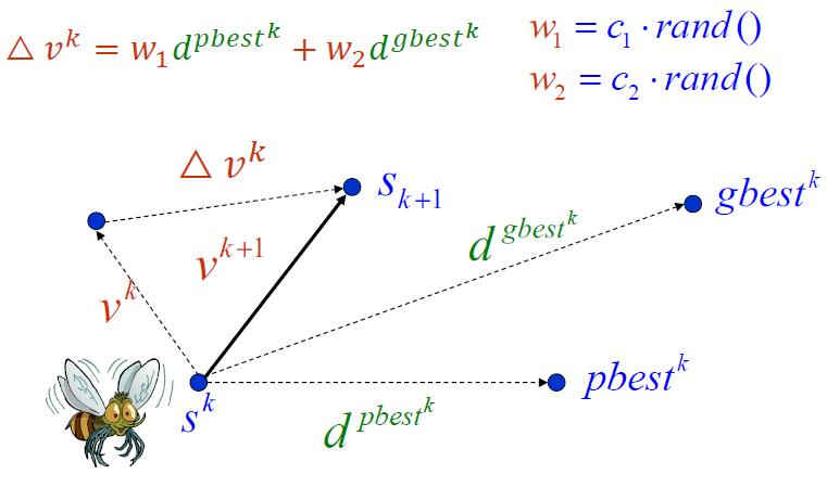
Simplified PSO algorithm
where
where
where
Flight vector influence
- Cognitive Component (
): Guides particles towards their personal best positions. - Social Component (
): Guides particles towards the global best position found by the swarm. - Inertia Weight (
): Balances exploration and exploitation, controlling the impact of the previous velocity on the current velocity.
Key Points
- PSO utilizes simple operations to explore the solution space efficiently.
- It balances exploration and exploitation by considering both personal and collective experiences.
- The method is known for its simplicity, ease of implementation, and ability to converge quickly to good solutions.
Particle Swarm Optimization offers a versatile and powerful approach for continuous optimization problems, leveraging the collective behavior observed in nature to yield effective results.
21. More Recent Swarm Intelligence Techniques: The Firefly Algorithm
The Firefly Algorithm, inspired by bioluminescent communication among fireflies, optimizes complicated functions by exploiting the mechanism of visual attraction. Each firefly's attractiveness is based on its brightness, which corresponds to the optimality of its solution.
Fireflies adjust their movements toward brighter counterparts, facilitating collective convergence to high-quality solutions. This algorithm is distinguished by its simplicity and effectiveness across varied optimization problems and is particularly adept at handling multimodal landscapes, offering a robust alternative to conventional optimization strategies with fewer control parameters.
Key Concepts
- Brightness: Represents the quality or fitness of a solution. Brighter fireflies attract others.
- Attractiveness: The attractiveness of a firefly is proportional to its brightness and decreases with distance.
- Movement: Fireflies are attracted to brighter ones and move towards them, which ideally leads them to higher quality solutions.
Formulas
Attractiveness
Absolute darkness is assumed.
Light intensity - Proportional to the quality of the solution. It decreases with distance according to:
where
Distance - The Euclidean distance between two fireflies:
where
Attractiveness - Dependent on initial light intensity
Movement - Firefly
where
Special cases
if
, then and the attractiveness is constant. - Absolute clear air, no absorption, no light dispersion.
- Each firefly can see each other regardless of the distance.
- Exploitation-exploitation balance is lost.
if
, then and the attractiveness is zero. - Absolute darkness, infinite absorption, no light reaches other fireflies.
- Fireflies cannot see each other.
- Random movement.
- Exploitation-exploitation balance is lost.
Applications
- Optimization Problems: Across fields like engineering and computer science.
- Data Clustering: Defining optimal groups in data.
- Image Processing: Improving feature extraction and segmentation.
Key Points
- The Firefly Algorithm leverages simple natural rules for optimization.
- Attractiveness and movement guide exploration in complex spaces.
- The algorithm efficiently handles multi-modal problems through dynamic interactions.
22. The Basics of Neural Networks
Neural networks consist of interconnected nodes (neurons) designed to approximate complex mathematical functions and model nonlinear relationships. Each node applies a weighted sum of inputs followed by an activation function, enabling the network to capture intricate patterns across layers.
These networks, particularly deep learning models, have revolutionized fields like image recognition, language processing, and autonomous systems by learning hierarchical feature representations. However, neural networks demand extensive data, computational resources, and careful architecture design to avoid overfitting and ensure generalizability.
Components
Artificial Neuron
Process input signals and apply an activation function to produce an output. A mimicking model for biological neuron.
- A neuron can only perform some simple information processing, therefore it is not able to solve complex problems.
- Neurons can be interconnected to deliver collective complex behavior and thus they can be used for solving complex problems
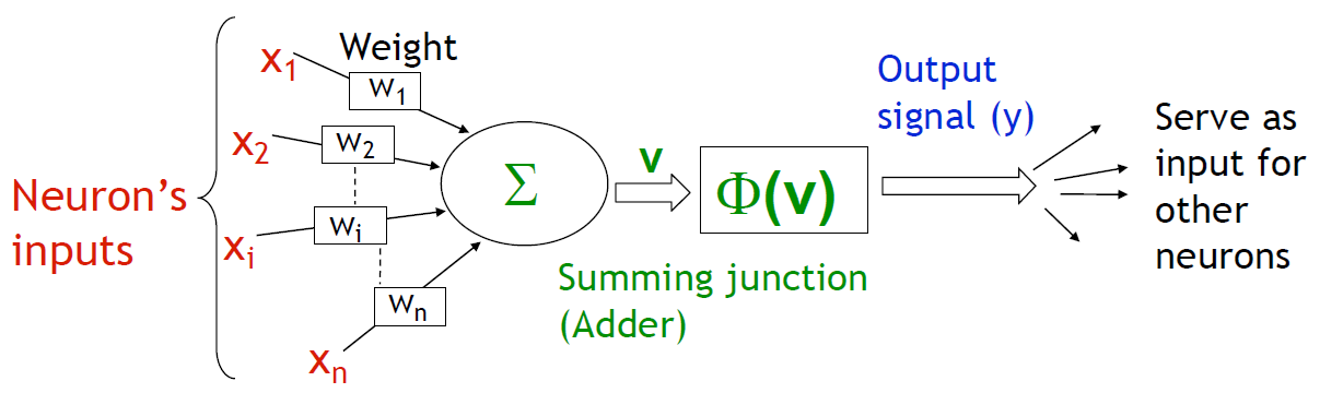
Activation Function
Determines the output of a neuron given an input or set of inputs. Common activation functions include
Limits the output between two asymptotes so that it can keep neuron output within reasonable dynamic range
Layers
- Input Layer: Receives input data and passes it to the hidden layers.
- Hidden Layers: Intermediate layers between the input and output layers where the network learns patterns.
- Output Layer: Produces the final output based on the learned patterns.
Weights and Biases
- Weights: Parameters that adjust the strength of connections between neurons.
- Biases: Additional parameters that shift the output of neurons.
Overview
| Biological Neuron | Artificial Neuron |
|---|---|
| Soma | Neuron |
| Dendrite | Input |
| Axon | Output |
| Synapse | Weight |
Key Points
- Neural networks model simulate the behavior of the human brain to solve complex problems.
- They consist of interconnected neurons that process information through layers.
- Effective with large datasets and sufficient computational resources.
- Foundation of deep learning techniques for various AI applications.
23. Perceptron: Perceptron Training
The perceptron is a fundamental building block of neural networks, acting as a binary classifier or a logic gate used for binary classification tasks, classifying linearly separable data. It combines input features, applies a weighted sum, and uses a step function to produce binary outputs.
Single Layer Perceptron
The single-layer perceptron is designed to address linearly separable patterns, where data can be divided into distinct classes using a straight line. This model initially led to disappointment in the 1970s because it was unable to solve non-linear problems such as XOR. However, this limitation spurred the development of multilayer perceptrons.
Linear separability means that you can separate data points with a straight line (or hyperplane in higher dimensions), which the perceptron can achieve with the equation:
Here,
Implementing Logic Gates
- Using McCulloch-Pitts Neurons: Construct basic logic gates (NOT, AND, OR) by setting appropriate weights and thresholds.
- Example Implementations:
- NOT Gate: Weight =
, Threshold = - AND Gate: Weights =
, Threshold = - OR Gate: Weights =
, Threshold =
- NOT Gate: Weight =
Training Process
Initialization:
- Randomly set weights
- Set threshold
and learning rate .
- Randomly set weights
Activation:
- Output calculated using:
Weight Training:
- Update weights:
- Correction:
- Error:
Iteration:
- Repeat until convergence or a set number of iterations.
Limitations
- Inability to solve non-linear separable problems like XOR without multilayered architecture.
- Challenges in determining weights and thresholds manually for complex networks.
The perceptron, while basic, is crucial for understanding more complex neural network architectures and serves as the foundation for learning binary classification tasks through supervised methods.
Example problem 1
Problem image
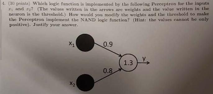
Determine which logic function is implemented by the following perceptron with inputs
Solution
The perceptron computes the weighted sum:
Input combinations:
: Output 0 : Output 0 : Output 0 : Output 1
Therefore, this configuration implements the AND logic function.
Modification for NAND Function
NAND outputs 1 for all inputs except
If we invert the sign of the weights and threshold, the perceptron will output 1 for the NAND function:
- For
: Output 0 - For all other inputs, the weighted sum is greater than -1.3, resulting in Output 1.
Example problem 2
A two-input perceptron tries to learn the OR logic function. In one phase of learning, the two weights of the perceptron are as follows:
Solution
Given
- weights:
, - threshold:
- learning rate:
Function to learn: OR, with a truth table:
Epoch process
For each input pair, we calculate the net input and predicted output, then update the weights if there's an error. The weight update uses the formula:
The error is calculated as the difference between desired output and predicted output.
Input
Net input calculation:
Predicted output:
- Since
, the output is 0.
- Since
Error calculation:
- Desired output: 0
- Error:
Weight update: No change
Input
Net input calculation:
Predicted output:
- Since
, the output is 0.
- Since
Error calculation:
- Desired output: 1
- Error:
Weight update:
Input
Net input calculation:
Predicted output:
- Since
, the output is 0.
- Since
Error calculation:
- Desired output: 1
- Error:
Weight update:
Input
Net input calculation:
Predicted output:
- Since
, the output is 0.
- Since
Error calculation:
- Desired output: 1
- Error:
Weight update:
Updated weights after 1 epoch
Key Points
- The perceptron is a basic neural network unit for binary classification tasks.
- It classifies linearly separable data using weighted inputs and a threshold.
- Training involves adjusting weights based on input-output discrepancies.
- Limitations include non-linear separability and manual weight setting for complex problems.
24. The Basic Concept of CRISP-DM
CRISP-DM (Cross-Industry Standard Process for Data Mining) is a widely used model for data mining projects, providing a structured approach to guide the project lifecycle.
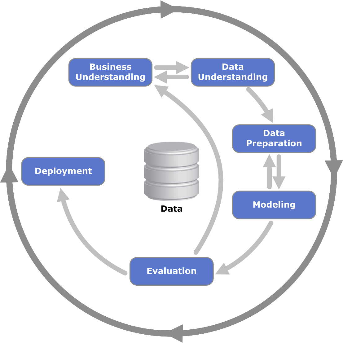
Phases of CRISP-DM
Business Understanding
- Define project objectives and requirements from a business perspective.
- Translate these into a data mining problem definition.
Data Understanding
- Collect initial data and get familiar with it.
- Identify data quality issues and discover initial insights.
Data Preparation
- Clean, construct, and format data into the final dataset.
- Perform tasks like data normalization, transformation, and feature selection.
Modeling
- Select appropriate modeling techniques and algorithms.
- Build and assess models, often requiring parameter tuning.
Evaluation
- Review model performance to ensure it meets the business objectives.
- Determine if there are important business issues not covered sufficiently.
Deployment
- Implement the model into the operational environment.
- Plan for monitoring and maintenance to ensure continued effectiveness.
Benefits
- Structured Approach: Provides a clear, repeatable process for data mining.
- Flexibility: Adaptable to various industries and project types.
- Focus: Keeps efforts aligned with business objectives throughout the project lifecycle.