
Introduction to Machine Learning (Topics 13 - 18)
13. The Q-learning method
Q-learning is a fundamental technique in reinforcement learning that enables agents to learn optimal actions through experience. By navigating its environment, the agent tries different actions and receives feedback in the form of rewards. This trial-and-error approach allows the agent to build a strategy that maximizes its cumulative rewards over time.
The strength of Q-learning is its ability to operate without a model of the environment, making it adaptable to complex situations. It uses a Q-table to track the quality of actions in each state, gradually guiding the agent towards better decisions.
Key Components of Q-learning
Q-table
The Q-table is a repository of rewards associated with optimal actions for each state in a given environment. It serves as a guide for the agent, helping it determine which actions are likely to yield the best outcomes. As the agent interacts with the environment, the Q-table is dynamically updated to reflect the agent’s evolving understanding, enabling more informed decision-making.
Q-Values or Action-Values
Stored in a Q-table, Q-values are associated with specific states and actions.
Methods for Determining Q-Values
There are two methods for determining Q-values:
Temporal Difference: Calculated by comparing the current state and action values with the previous ones.
Bellman’s Equation: A recursive formula invented by Richard Bellman in 1957, used to calculate the value of a given state and determine its optimal position. It provides a recursive formula for calculating the value of a given state in a Markov Decision Process (MDP) and is particularly influential in the context of Q-learning and optimal decision-making.
Rewards
In Q-learning, an agent navigates through various states by selecting actions based on its current state and the surrounding environment. At each step, the agent receives a reward from the environment, which serves as feedback for its action. The reward indicates how favorable the action was in achieving the agent's goals. The episode ends when the agent reaches a terminal state where no further transitions are possible.
The total reward, denoted as (R_t), is the sum of all rewards received from time (t), discounted over time. This is calculated as:
Here,
Temporal Difference (Update Rule)
The Temporal Difference or TD-Update rule can be represented as follows:
This update rule to estimate the value of
and represent the current state and action. is the next state after taking action in state . is next best action to be picked using current Q-value estimates. is the immediate reward received after taking action in state . is the learning rate, determining the extent to which new information overrides old information. is the discount factor, balancing immediate and future rewards.
The TD-Update rule is crucial for updating the Q-values based on the observed rewards and the agent's predictions. It helps the agent learn the optimal policy by iteratively refining its estimates of the Q-values.
Exploration-Exploitation Dilemma
One of the key challenges in reinforcement learning is the exploration-exploitation trade-off. The agent must balance between exploring new actions to discover potentially better strategies and exploiting known actions that have yielded high rewards in the past. Q-learning often employs strategies like
Superior Q-Value Action (Exploitation)
- With a probability of
, representing the majority of cases - Select the action with the highest Q-value at the moment
- In this instance of exploitation, the agent chooses the course of action that, given its current understanding, it feels is optimal
Exploration through Random Action (Exploration)
- With a probability of
, representing a small fraction of cases - Rather than selecting the course of action with the highest Q-value, the agent chooses a random action
- Select any action at random, regardless of its Q-value
- This random selection allows the agent to explore new possibilities and potentially discover better strategies
Advantages and Disadvantages of Q-learning
Advantages
- Model-Free: No need for a predefined model of the environment.
- Effective in Discrete Spaces: Works well in environments with distinct states and actions.
Disadvantages
- Scalability: Struggles in high-dimensional or continuous spaces due to the exponential growth of state-action pairs.
- Convergence: May require extensive training to converge to optimal policies.
Key Points
- Q-learning is a model-free reinforcement learning algorithm that learns optimal policies through trial-and-error.
- Components of Q-learning include the Q-table, Q-values, rewards, and the Temporal Difference update rule.
- The exploration-exploitation dilemma is addressed using strategies like
-greedy. - Q-learning is effective in discrete environments but faces challenges in scalability and convergence.
14. Deep Learning Methods: Value Learning and Policy Learning
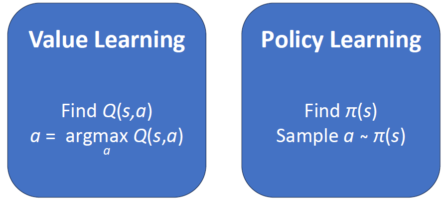
Deep learning extends reinforcement methods to complex tasks by incorporating neural networks, enabling more efficient learning of value functions (value learning) and policies (policy learning). Value learning estimates cumulative rewards for states, while policy learning focuses on optimal action selections.
Deep reinforcement learning utilizes architectures like deep Q-networks (DQNs) for discrete action spaces, and policy-based methods like Policy Gradient.These techniques empower AI to handle intricate environments but require substantial computational resources and careful hyperparameter tuning to ensure stability and convergence.
Main Types of Deep Reinforcement Learning Algorithms
Value-Based Methods
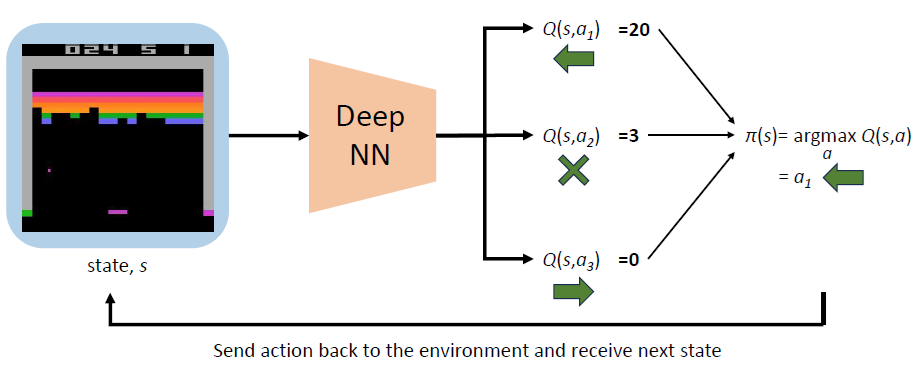
Value-based methods focus on learning the value of actions given states. The Q-values inform which actions maximize expected long-term rewards. Deep Q-Networks (DQNs) are a popular example of value-based methods that leverage deep neural networks to approximate the Q-values efficiently.
- Main idea: Approximate Q function and use it to infer the optimal policy.
- Example: Deep Q-Networks (DQN).
Policy-Based Methods
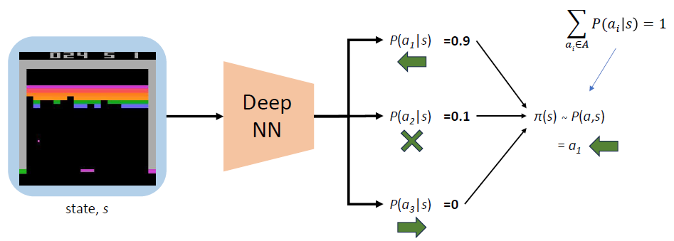
Policy-based methods directly learn the policy mapping states to actions. This approach optimizes the policy itself, allowing the agent to determine the best action in each state without estimating a value function.
- Main idea: Directly optimize the policy to maximize expected rewards.
- Example: Policy Gradient Methods.
Preferences for Value-Based vs. Policy-Based Methods
In reinforcement learning, choosing between value-based and policy-based methods depends on the problem's nature and specific requirements.
When to Prefer Value-Based Methods
- Discrete Action Spaces: Value-based methods like Deep Q-Networks (DQN) are well-suited for environments with a limited number of discrete actions.
- Efficiency: These methods are efficient when the state and action spaces are not prohibitively large, as they focus on estimating the value function to guide decision-making.
- Stable Learning: Value-based techniques can be more stable as they directly estimate the value of actions to derive policies.
- Optimality: If the environment's dynamics allow for a precise estimation of state-action values, value-based methods can effectively determine optimal policies.
When to Prefer Policy-Based Methods
- Continuous Action Spaces: Policy-based methods excel in environments with continuous actions, where discretizing actions would be impractical or infeasible.
- High-Dimensional Action Spaces: These methods directly learn a policy, avoiding the need to evaluate a vast number of potential actions.
- Stochastic Policies: Useful when the optimal solution requires a stochastic policy (meaning actions are chosen probabilistically).
- Exploration Challenges: Policy gradients can better explore the action space, as they adjust the policy directly rather than relying on discrete value evaluations.
Key Points
- Deep reinforcement learning combines neural networks with reinforcement learning to handle complex tasks.
- Value-based methods like DQNs estimate action values, while policy-based methods directly optimize policies.
- Policy gradients optimize policies by adjusting parameters to maximize expected rewards.
- Value-based methods are efficient in discrete spaces, while policy-based methods excel in continuous or high-dimensional spaces.
- The choice between value-based and policy-based methods depends on the problem's characteristics and requirements.
15. The Policy Gradient Algorithm
The Policy Gradient algorithm is a key method in reinforcement learning that directly optimizes the policy function. Unlike value-based methods, which derive a policy implicitly by estimating value functions, policy gradient methods learn a parameterized policy that maps states directly to actions. This approach is particularly advantageous in environments with continuous or high-dimensional action spaces.
Training Policy Gradients
Policy gradient algorithms aim to maximize expected cumulative rewards by adjusting the policy's parameters using feedback from the environment. They employ stochastic gradient ascent to optimize these parameters, adapting the policy based on observed rewards from interacting with the environment.
Training Algorithm
- Initialize the Agent: Start with a randomly initialized policy.
- Run the Policy: Execute the current policy in the environment until an episode concludes.
- Record Data: Collect data on states, actions, and rewards experienced.
- Update Probabilities:
- Decrease Probability of Low-Reward Actions: Adjust the policy to reduce the likelihood of actions with lower rewards.
- Increase Probability of High-Reward Actions: Enhance the probability of actions that yield higher rewards.
- Repeat: Iterate through steps 2-5, continuously improving the policy.
Loss and Gradient Descent in Policy Gradients
Loss Function
- The loss function gauges the performance of the policy. It is generally defined in terms of the expected return of actions taken under the policy.
- The aim is to minimize this loss to refine policy performance. Typically, the loss is expressed as the negative log-probability of actions taken, scaled by the received rewards. This formulation helps in understanding how changes in policy parameters impact expected rewards.
Gradient Descent
Policy gradient methods utilize stochastic gradient ascent (a variant of gradient descent) since they maximize rather than minimize the expected rewards.
- Gradient Descent: An optimization technique to find the minimum of a loss function by iteratively adjusting parameters in the direction of the steepest descent.
- Gradient Ascent: Applied in policy gradients as the objective is to maximize rewards by moving parameters in the direction of the gradient’s increase.
Updating the Policy:
- The policy parameters are updated using calculated gradients to increase expected returns. This involves computing the derivative of expected reward concerning policy parameters and making appropriate adjustments:
: Policy parameters. : Learning rate, governing the step size for each adjustment. : Probability of taking action in state under policy . : Reward signal.
By continually adjusting the policy parameters, the agent enhances its decision-making abilities, favoring actions that lead to higher rewards, and gradually improving its performance in the given environment.
Key Points
- Policy gradients adjust policy parameters to maximize expected cumulative rewards.
- The loss function quantifies policy performance, guiding parameter updates.
- Stochastic gradient ascent is used to optimize policy parameters by moving in the direction of increased expected rewards.
16. The Basic Concept of Evolutionary Algorithms
Evolutionary algorithms are optimization techniques inspired by the process of natural selection. They iteratively evolve solutions using biological mechanisms such as selection, crossover, and mutation. These algorithms are ideal for handling complex optimization problems where traditional methods struggle.
Key Concepts
- Gene: Functional entity encoding a specific feature of the individual (e.g., hair color).
- Allele: The specific value of a gene (e.g., blonde).
- Genotype: The combination of alleles carried by an individual.
- Phenotype: The physical manifestation of an organism.
- Locus: The position of the gene within the chromosome.
- Individual: Represents a candidate solution, often modeled as a chromosome.
Evolutionary Algorithms
- Their basic principle is the search on the population of solutions guided by laws known from biology
- The individuals in the population are the solutions of the given problem
- The population is evolving, we obtain better and better individuals
Advantages
- Robustness: Able to find good solutions even in complex, multimodal landscapes.
- Adaptability: Can automatically adjust to changes in the optimization problem.
- Scalability: Performs well in large, high-dimensional spaces.
Key Points
- Evolutionary algorithms are optimization techniques inspired by natural selection.
- Evolutionary algorithms iterate over generations, refining the population toward optimal solutions.
- They balance exploration and exploitation through genetic diversity and fitness-guided selection.
- The adaptability and robustness of evolutionary algorithms make them suitable for a wide range of complex scenarios.
17. Optimization by Genetic Algorithm
Genetic algorithms (GAs) are a subset of evolutionary algorithms that specifically use genetic operators to evolve solutions for optimization problems. Inspired by the principles of natural selection and genetics, GAs iteratively improve candidate solutions by mimicking biological processes like selection, crossover, and mutation.
Key Concepts
- Population: Collection of individuals currently alive in the algorithm.
- Fitness Function: A measure to evaluate how well a solution solves the problem, guiding the selection of the best candidates.
- Selection: The process of choosing superior solutions from the current population based on their fitness scores.
- Crossover (Recombination): Combining parts of two or more parent solutions to create offspring that inherit traits from each parent.
- Mutation: Introducing random alterations to solutions to maintain diversity within the population and explore new solution spaces.
Genetic Algorithm Process
Initialization: Generate an initial population of solutions randomly.
Evaluation: Assign fitness scores to each solution based on the fitness function.
Selection: Choose the fittest individuals for reproduction.
- Roulette Wheel Selection: Individuals are chosen based on fitness proportion. Better chromosomes have a higher chance of selection, analogous to a roulette where the ball lands according to fitness proportions.
Crossover: Create offspring through the recombination of selected individuals.
- Choose a random crossover point in parent chromosomes.
- Split the parents at this point.
- Create offspring by exchanging tails.
- Ensures genetic diversity in the next generation.
Mutation: Apply random mutations to some offspring to introduce variation.
- Each gene may mutate independently with a specified probability (e.g., 5%).
- This introduces new genetic variations, helping the algorithm explore new solution spaces.
Replacement: Form a new generation by replacing some or all of the old population with the new offspring.
Termination: Continue iterations until a stopping criterion is reached, such as a solution meeting the desired fitness or reaching a maximum number of generations.
Example
Given the following population of binary strings:
, fitness: 5 , fitness: 27 , fitness: 30 , fitness: 33 , fitness: 5 , fitness: 100
Using roulette wheel selection, calculate the expected number of copies of each individual in the crossover while maintaining a constant population size. Illustrate the crossover with the selected individuals and show mutation with a 5% per bit mutation probability.
Solution
In this example initialization and evaluation are assumed to have been completed, and the fitness values are known.
- Selection:
- Total Fitness:
- Calculate each individual’s probability using their fitness over total fitness.
- Expected number of copies for each individual:
Based on calculated probabilities, select 6 parents.
Likely selection based on probabilities:
(3 times) (1 time) (1 time) (1 time)
- Crossover:
- Perform crossover between selected parents to create offspring.
Selected parents:
Using a random crossover point, let's choose position 4 (splitting after the 4th bit) for illustration:
Pair 1:
and - Parent 1:
- Parent 2:
- Offspring 1: take
and : - Offspring 2: take
and :
- Parent 1:
Pair 2:
and - Parent 1:
- Parent 2:
- Offspring 1: take
and : - Offspring 2: take
and :
- Parent 1:
Pair 3:
and - Parent 1:
- Parent 2:
- Offspring 1: take
and : - Offspring 2: take
and :
- Parent 1:
Therefore, the offspring after crossover are:
- Mutation:
Given a 5% mutation probability per bit, since we have 48 bits in total (6 individuals with 8 bits each), on average we can expect approximately 2-3 bits to mutate.
Let's assume the following bits mutate:
: stays unchanged : 4th bit changes : 6th bit changes : stays unchanged : 8th bit changes : stays unchanged
- Replacement:
Replace the old population with the new offspring. Since the population size remains constant, the new generation consists of the offspring generated through crossover and mutation.
Result after one iteration:
Key Points
- Genetic algorithms use genetic operators like selection, crossover, and mutation to evolve solutions.
- The roulette wheel selection method is commonly used to select parents based on their fitness scores.
- Crossover combines genetic material from parents to create offspring, maintaining genetic diversity.
- Mutation introduces random changes to offspring to explore new solution spaces and prevent premature convergence.
18. The Basic Concept of Genetic Programming: Differences Compared to Genetic Algorithms
Genetic programming extends genetic algorithms to evolve entire programs or symbolic expressions, enabling computers to automatically create software solutions for tasks without human intervention. It adapts genetic principles but evolves dynamic structures like code or mathematical functions rather than fixed-length candidate solutions.
Key features of Genetic Programming:
Representation - In GP, candidate solutions are typically represented as tree structures, where:
- Internal nodes represent functions (e.g., mathematical operations like +, -, *, /, or logical operations like AND, OR)
- Leaf nodes represent variables, constants, or inputs to the problem
- Trees can vary in size and complexity, allowing for the evolution of diverse solutions
Evolutionary Process - GP follows the same evolutionary process as genetic algorithms, including:
- Initialization of a population of random programs
- Evaluation of programs based on their fitness
- Selection of programs for reproduction based on fitness
- Crossover and mutation to create new programs
- Replacement of old programs with new offspring
Output - The output of GP is a program or function that solves the given problem. This program can be executed
Differences between Genetic Programming and Genetic Algorithms
| Aspect | Genetic Programming (GP) | Genetic Algorithms (GA) |
|---|---|---|
| Solution Representation | Programs or expressions (tree structures) | Fixed-length chromosomes (binary, real-valued, etc.) |
| Output | A program, function, or expression | An optimized solution or parameter set |
| Primary Goal | Evolve executable structures (programs) | Optimize predefined parameters |
| Mutation and Crossover | Operate on program trees (subtrees) | Operate on fixed-length chromosomes |
| Application Focus | Symbolic regression, program generation, etc. | Optimization problems like feature selection, weight tuning, etc. |
| Complexity of Solutions | Solutions can be dynamic and variable-length (tree size may grow) | Fixed-size solutions, defined by chromosome length |
Example Comparison
GP Example
- Problem: Automatically discover a trading algorithm for a stock market.
- Representation: Each program (tree) encodes a decision-making algorithm for buying or selling stocks.
- Fitness: Profit generated by the algorithm in a simulated environment.
- Output: A fully functional trading algorithm.
GA Example
- Problem: Optimize hyperparameters for a trading algorithm.
- Representation: Chromosomes encode parameters like learning rate, stop-loss percentage, etc.
- Fitness: Performance of the algorithm using those parameters.
- Output: An optimized set of hyperparameters.
Key Points
- Genetic Programming evolves programs or functions to solve problems.
- Solutions are represented as tree structures, allowing for variable-length and complex solutions.
- Key differences between GP and GAs is that GP evolves programs, while GAs optimize fixed-length solutions.